Kappa
“Great things are not done by impulse, but by a series of small things brought together.”
Hack The Box
Neural Networks
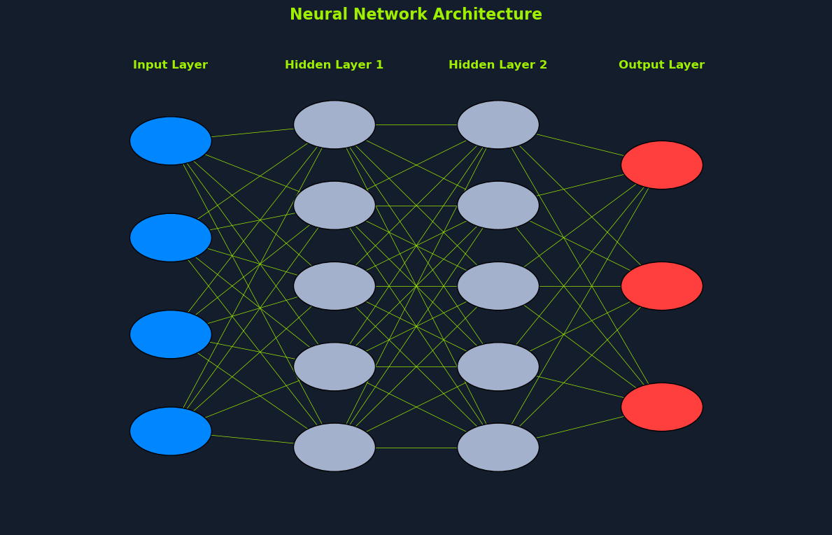
To overcome the limitations of single-layer perceptrons, we introduce the concept of neural networks with multiple layers. These networks, also known as multi-layer perceptrons (MLPs), are composed of:
- An input layer
- One or more hidden layers
- An output layer
Neurons
A neuron is a fundamental computational unit in neural networks. It receives inputs, processes them using weights and a bias, and applies an activation function to produce an output. Unlike the perceptron, which uses a step function for binary classification, neurons can use various activation functions such as the sigmoid, ReLU, and tanh.
This flexibility allows neurons to handle non-linear relationships and produce continuous outputs, making them suitable for various tasks.
Input Layer
The input layer serves as the entry point for the data. Each neuron in the input layer corresponds to a feature or attribute of the input data. The input layer passes the data to the first hidden layer.
Hidden Layers
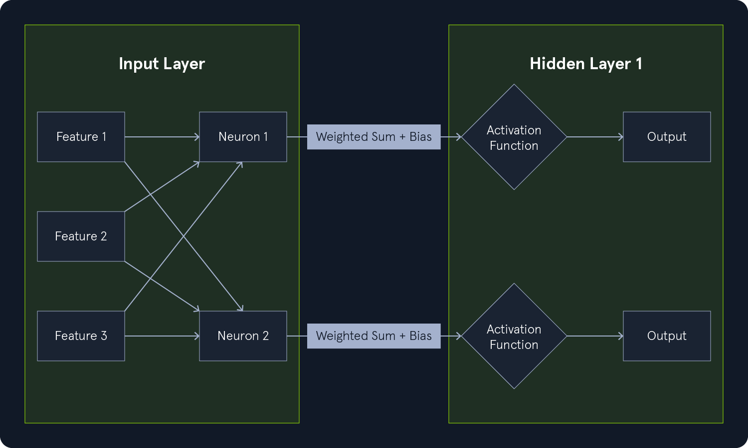
Hidden layers are the intermediate layers between the input and output layers. They perform computations and extract features from the data. Each neuron in a hidden layer:
- Receives input from all neurons in the previous layer.
- Performs a weighted sum of the inputs.
- Adds a bias to the sum.
- Applies an activation function to the result.
The output of each neuron in a hidden layer is then passed as input to the next layer.
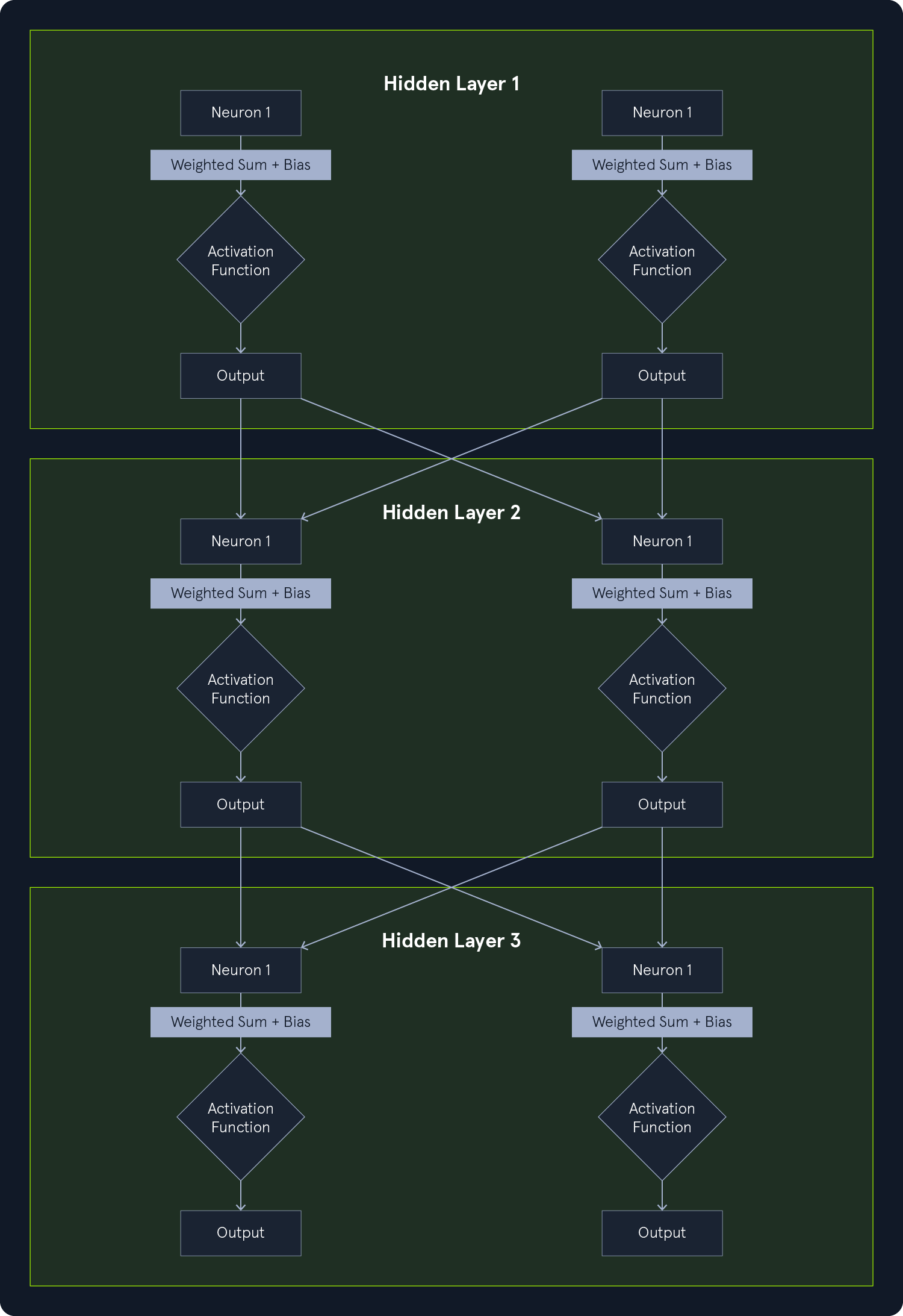
Multiple hidden layers allow the network to learn complex non-linear relationships within the data. Each layer can learn different levels of abstraction, with the initial layers learning simple features and subsequent layers combining those features into more complex representations.
Output Layer
The output layer produces the network's final result. The number of neurons in the output layer depends on the specific task:
- A binary classification task would have one output neuron.
- A multi-class classification task would have one neuron for each class.
The Power of Multiple Layers
Multi-layer perceptrons (MLPs) overcome the limitations of single-layer perceptrons primarily by learning non-linear decision boundaries. By incorporating multiple hidden layers with non-linear activation functions, MLPs can approximate complex functions and capture intricate patterns in data that are not linearly separable.
This enables them to solve problems like the XOR problem, which single-layer perceptrons cannot address. Additionally, the hierarchical structure of MLPs allows them to learn increasingly complex features at each layer, leading to greater expressiveness and improved performance in a broader range of tasks.
Activation Functions
Activation functions play a crucial role in neural networks by introducing non-linearity. They determine a neuron's output based on its input. Without activation functions, the network would essentially be a linear model, limiting its ability to learn complex patterns.
Each neuron in a hidden layer receives a weighted sum of inputs from the previous layer plus a bias term. This sum is then passed through an activation function, determining whether the neuron should be "activated" and to what extent. The output of the activation function is then passed as input to the next layer.
Types of Activation Functions
There are various activation functions, each with its own characteristics and applications. Some common ones include:
- Sigmoid: - The sigmoid function squashes the input into a range between 0 and 1. It was historically popular but is now less commonly used due to issues like vanishing gradients.
- ReLU (Rectified Linear Unit): - ReLU is a simple and widely used activation function. It returns 0 for negative inputs and the input value for positive inputs. ReLU often leads to faster training and better performance.
- Tanh (Hyperbolic Tangent): - The tanh function squashes the input into a range between -1 and 1. It is similar to the sigmoid function but centered at 0.
- Softmax: - The softmax function is often used in the output layer for multi-class classification problems. It converts a vector of raw scores into a probability distribution over the classes.
The choice of activation function depends on the specific task and network architecture.
Training MLPs
Training a multi-layer perceptron (MLP) involves adjusting the network's weights and biases to minimize the error between its predictions and target values. This process is achieved through a combination of backpropagation and gradient descent.
Backpropagation
Backpropagation is an algorithm for calculating the gradient of the loss function concerning the network's weights and biases. It works by propagating the error signal back through the network, layer by layer, starting from the output layer.
Here's a simplified overview of the backpropagation process:
- Forward Pass: - The input data is fed through the network, and the output is calculated.
- Calculate Error: - A loss function calculates the difference between the predicted output and the actual target value.
- Backward Pass: - The error signal is propagated back through the network. For each layer, the gradient of the loss function concerning the weights and biases is calculated using the calculus chain rule.
- Update Weights and Biases: - The weights and biases are updated to reduce errors. This is typically done using an optimization algorithm like gradient descent.
Gradient Descent
Gradient descent is an iterative optimization algorithm used to find the minimum of a function. In the context of MLPs, the loss function is minimized.
Gradient descent works by taking steps toward the negative gradient of the loss function. The size of the step is determined by the learning rate, a hyperparameter that controls how quickly the network learns.
Here's a simplified explanation of gradient descent:
- Initialize Weights and Biases: - Start with random values for the weights and biases.
- Calculate Gradient: - Use backpropagation to calculate the gradient of the loss function with respect to the weights and biases.
- Update Weights and Biases: - Subtract a fraction of the gradient from the current weights and biases. The learning rate determines the fraction.
- Repeat: - Repeat steps 2 and 3 until the loss function converges to a minimum or a predefined number of iterations is reached.
Backpropagation and gradient descent work together to train MLPs. Backpropagation calculates the gradients, while gradient descent uses those gradients to update the network's parameters and minimize the loss function. This iterative process allows the network to learn from the data and improve its performance over time.
Fundamentals of AI
- Introduction to Machine Learning
- Mathematics Refresher for AI
- Supervised Learning Algorithms
- Linear Regression
- Logistic Regression
- Decision Trees
- Naive Bayes
- Support Vector Machines (SVMs)
- Unsupervised Learning Algorithms
- K-Means Clustering
- Principal Component Analysis (PCA)
- Anomaly Detection
- Reinforcement Learning Algorithms
- Q-Learning
- SARSA (State-Action-Reward-State-Action)
- Introduction to Deep Learning
- Perceptrons
- ~ Neural Networks
- Convolutional Neural Networks